05
Mar
The general rule of thumb to use normal approximation to binomial distribution is that the sample size n is sufficiently large if n p 5 and n 1 p 5. Suppose we have say n independent trials of this same experiment.

Normal approximation to the binomial. It turns out that if n is sufficiently large then we can actually use the normal distribution to approximate the probabilities related to the binomial distribution. This is known as the normal approximation to the binomial. For n to be sufficiently large it.
By the way you might find it interesting to note that the approximate normal probability is quite close to the exact binomial probability. We showed that the approximate probability is 00549 whereas the following calculation shows that the exact probability using the binomial table with n10 and pfrac12 is 00537. The general rule of thumb to use normal approximation to binomial distribution is that the sample size n is sufficiently large if n p 5 and n 1 p 5.
For sufficiently large n X N μ σ 2. That is Z X μ σ X n p n p 1 p N 0 1. The approximate normal distribution has parameters corresponding to the mean and standard deviation of the binomial distribution.
µ np and σ np1 p The normal approximation may be used when computing the range of many possible successes. For instance we may apply the normal distribution to the setting of the previous example. The actual binomial probability is 01094 and the approximation based on the normal distribution is 01059.
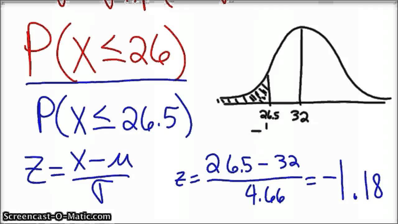
Note that the normal approximation computes the area between 55 and 65 since the probability of getting a value of exactly 6 in a continuous distribution is nil. Similarly to approximate the probability of from 0 to 6 successes you. Normal Approximation to the Binomial 1.
Sum of many independent 01 components with probabilities equal p with n large enough such that npq 3 then the binomial number of success in n trials can be approximated by the Normal distribution with mean µ np and standard deviation q np1p. Chapter 5 Normal approximation to the Binomial log bk max 1 bk max log bk max 2 bk max 1 log bk max m bk max m 1 1 2 m npq 1 2 m2 npq. Thus PX k max mbk maxexp m2 2npq for m not too large.
An analogous approximation holds for 0 k max m k max. The general rule of thumb to use normal approximation to binomial distribution is that the sample size n is sufficiently large if np 5 and n1 p 5. For sufficiently large n X Nμ σ2.
That is Z X μ σ X np np 1 p N0 1. The normal approximation means that you can use the normal distribution as an approximation to calculate the probabilities for binomial distribution. Note that this can be done under the following conditions.
The number of trials n is large. Generally values of n greater than 30 are considered to be large. The Bernoulli random variable is a special case of the Binomial random variable where the number of trials is equal to one.
Suppose we have say n independent trials of this same experiment. Then we would have n values of Y namely Y_1 Y_2 Y_n. If we define X to be the sum of those values we get.
The normal distribution is generally considered to be a pretty good approximation for the binomial distribution when np 5 and n1 p 5. For values of p close to 5 the number 5 on the right side of these inequalities may be reduced somewhat while for more extreme values of p especially for p 1 or p 9 the value. When this is the case we can use the normal curve to estimate the various probabilities associated with that binomial distribution.
For example P binomial 5 x 10 can be approximated by P normal 55 x 95. Similarly P binomial 10 can be approximated by P normal 95 x 105. If you need a between-two-values probability that is p a X b do Steps 14 for b the larger of the two values and again for a the smaller of the two values and subtract the results.
When using the normal approximation to find a binomial probability your answer is an approximation not exact be sure to state that. Use the normal approximation to the binomial with n 10 and p 05 to find the probability P X 7. N 10 and p 05 so we first check to see if the normal approximation is appropriate.
N p 5 5 and n q 5 5 so it is. Then for the approximating normal distribution μ n p 5 and σ n p q 15811. 5 and 15 heads for a normal distribution with mean 8 and standard deviation 4.
Approximating the Binomial distribution Now we are ready to approximate the binomial distribution using the normal curve and using the continuity correction. Example 5 Suppose 35 of all households in Carville have three cars what is the probabil-. And since were using a normal appoximation of a binomial distribution we have to calculate from 465 to 475 z_1 frac465-505 -07 z_2 frac475-505.
That said you are probably asking for a better approximation to the binomial distribution in the sense of having more higher-order terms. I dont know whether the tail bounds on Wikipedia would help you since Im not familiar with them. Chapter 6 Normal Approximation to Binomial Lecture 4 Section.
66 Normal Approximation to Binomial Recall from Chapter 5 the Binomial Probability Distributions. The problem involves a binomial distribution with a large value of n and so very tedious arithmetic may be expected. This can be avoided by using the normal distribution to approximate the binomial distribution underpinning the problem.
If X represents the number of engineering students in favour of studying statistics then X B1000075.
Previous post
Normally open check valve